Wednesday 28 November 2012

The Failure of Mathematics?

Mathematics has come in for criticism recently, that somehow it was the root cause of the credit crunch and the collapse of the world economy. It was the misuse of mathematics, by bosses who didn’t understand it, that got us into the mire.

Actually, bosses do possess the tools; they simply refuse to use them. And then we wonder when it goes wrong.

The refusal to take mathematics seriously is the cause of all sorts of errors.

We assume things are static when they are dynamic.
We assume relationships between variables to be linear (and predictable) when they are not.
We ignore ranges of possibility and use single-point average values instead—the flaw of averages.
We assume that different uncertainties are independent, and get caught by surprise when we discover they are not.
We confuse cause and symptom and treat the latter, and are surprised when the former does not go away.
We assume that absence of evidence is evidence of absence.
We let vanishingly small risks bias our perception of the world (and let unwarranted fear guide our behavior), whilst ignoring the everyday risks that kill lots of us all the time.

The mathematics is sound. It’s the application that’s at fault. The failure of mathematicians—but not, —is to let get away with it.

Friday 2 November 2012

Worksheets IGCSE and O Level Mathematics

Worksheets

IGCSE

Mathematics

Note: Worksheet & Resource Pack is available on Separate topic
Price per topic = US $1
Send you mail order on :
Accountmatics@ymail.com

SHEETS

Extended

Trigonometry, Circle, Bearing
Click

Locus, Coordinate Geometry, Vector
Click

Locus and Coordinate Geometry
Click

Core

Statistics with Tally

Click

Mensuration with Unit Cost

Click

Sequences

Click

Algebra - Factorization, Subject, Indices

Click

Transformation

Click

Equation

Click

Perimeter

Click

Bearing

Click

Locus

Click

PAST PAPERS WITH MARK SCHEME

(2005-2012)

IGCSE
Click

Thursday 18 October 2012

MATHEMATICS - KEY POINTS

MATHEMATICS

KEY POINTS

EXAM GUIDE

GCE O LEVEL

Click Here

Wednesday 12 September 2012

IGCSE PAST PAPERS (Maths)

IGCSE

PAST PAPERS

MATHEMATICS
580

TOPICAL

PROBABILITY

Read

IN-EQUALITY

Read

VEN DIAGRAM

Read

JUNE 2006

READ

Sunday 9 September 2012

Simplex Method

Simplex algorithm

In mathematical optimization, Dantzig's simplex algorithm (or simplex method) is a popular algorithm for linear programming.The journal Computing in Science and Engineering listed it as one of the top 10 algorithms of the twentieth century .

Example

Consider the linear program

Minimize

$Z = -2 x - 3 y - 4 z\,$

Subject to

$\begin{align} 3 x + 2 y + z &= 10\\ 2 x + 5 y + 3 z &= 15\\ x,\, y,\, z &\ge 0 \end{align}$

This is represented by the (non-canonical) tableau

$\begin{bmatrix} 1 & 2 & 3 & 4 & 0 \\ 0 & 3 & 2 & 1 & 10 \\ 0 & 2 & 5 & 3 & 15 \end{bmatrix}$

Introduce artificial variables u and v and objective function W = u + v, giving a new tableau

$\begin{bmatrix} 1 & 0 & 0 & 0 & 0 & -1 & -1 & 0 \\ 0 & 1 & 2 & 3 & 4 & 0 & 0 & 0 \\ 0 & 0 & 3 & 2 & 1 & 1 & 0 & 10 \\ 0 & 0 & 2 & 5 & 3 & 0 & 1 & 15 \end{bmatrix}$

Note that the equation defining the original objective function is retained in anticipation of Phase II. After pricing out this becomes

$\begin{bmatrix} 1 & 0 & 5 & 7 & 4 & 0 & 0 & 25 \\ 0 & 1 & 2 & 3 & 4 & 0 & 0 & 0 \\ 0 & 0 & 3 & 2 & 1 & 1 & 0 & 10 \\ 0 & 0 & 2 & 5 & 3 & 0 & 1 & 15 \end{bmatrix}$

Select column 5 as a pivot column, so the pivot row must be row 4, and the updated tableau is

$\begin{bmatrix} 1 & 0 & \tfrac{7}{3} & \tfrac{1}{3} & 0 & 0 & -\tfrac{4}{3} & 5 \\ 0 & 1 & -\tfrac{2}{3} & -\tfrac{11}{3} & 0 & 0 & -\tfrac{4}{3} & -20 \\ 0 & 0 & \tfrac{7}{3} & \tfrac{1}{3} & 0 & 1 & -\tfrac{1}{3} & 5 \\ 0 & 0 & \tfrac{2}{3} & \tfrac{5}{3} & 1 & 0 & \tfrac{1}{3} & 5 \end{bmatrix}$

Now select column 3 as a pivot column, for which row 3 must be the pivot row, to get

$\begin{bmatrix} 1 & 0 & 0 & 0 & 0 & -1 & -1 & 0 \\ 0 & 1 & 0 & -\tfrac{25}{7} & 0 & \tfrac{2}{7} & -\tfrac{10}{7} & -\tfrac{130}{7} \\ 0 & 0 & 1 & \tfrac{1}{7} & 0 & \tfrac{3}{7} & -\tfrac{1}{7} & \tfrac{15}{7} \\ 0 & 0 & 0 & \tfrac{11}{7} & 1 & -\tfrac{2}{7} & \tfrac{3}{7} & \tfrac{25}{7} \end{bmatrix}$

The artificial variables are now 0 and they may be dropped giving a canonical tableau equivalent to the original problem:

$\begin{bmatrix} 1 & 0 & -\tfrac{25}{7} & 0 & -\tfrac{130}{7} \\ 0 & 1 & \tfrac{1}{7} & 0 & \tfrac{15}{7} \\ 0 & 0 & \tfrac{11}{7} & 1 & \tfrac{25}{7} \end{bmatrix}$

This is, fortuitously, already optimal and the optimum value for the original linear program is −130/7.

EXAMPLE (Part 1): Simplex method

Resolve using the Simplex Method the following problem:

Maximize	Z = f(x,y) = 3x + 2y
subject to:	2x + y ≤ 18
	2x + 3y ≤ 42
	3x + y ≤ 24
	x ≥ 0 , y ≥ 0

Are considerated the following phases:

1. Turning the inequalities into equalities

Introduce a slack variable for each restrictions of the type ≤ to turn them into equalities, giving the following linear equation system:

2x + y + r = 18

2x + 3y + s = 42

3x +y + t = 24

2. Equaling the objective function to zero

- 3x - 2y + Z = 0

3. Writing the initial board simplex

At columns will appear all basic variables of the problem and the slack/surplus variables. At rows you can observe, for each restriction the slack variables with its coefficients of obtained equalities, and the last row with the values resulting of substitute the value of every variable at function objetive, and operate just as was explained in the theory to get the left values from the row:

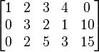
Board I . 1st iteration
			3	2	0	0	0
Base	Cb	P0	P1	P2	P3	P4	P5
P3	0	18	2	1	1	0	0
P4	0	42	2	3	0	1	0
P5	0	24	3	1	0	0	1
Z		0	-3	-2	0	0	0

4. Halt condition

When at the Z row there aren't negatives values , the optimal solution of the problem has been reached. In such a case, the algorithm has finished. If it were not so, the following steps must be executed.

5. Input-output base condition

A. First, we must know the variable that enters into the base. For it we choose that value's column that in the row the Z is the minor of the presents negatives values. In this case would be the variable x (P1) of coefficient - 3.

If two or more equal coefficients exist that obey the previous condition (tie case), then we will choose that variable that be basic.

The column of the variable that goes into the base is named pivot column (In green color).
Once the variable that goes into the base was obtained, we are in condition to deduce what will be the variable that goes out . For it, divide each independent term (P0) among the correspondent element of the pivot column, taking care that the result must be bigger than zero, and the minimum of this values is chosen.

In our case: 18/2 [=9] , 42/2 [=21] y 24/3 [=8]

If any less or equal to zero element exist, such divide will not be do, or if every elements that belongs to pivot column are zero we are in the case of unbounded solution, and the problem just would be finished (See theory).

The term of the pivot column that gives the lowest positive quotient in previous division, the 3, right now than 8 is the lower quotient, indicates the row of the slack variable that goes out the base, t (P5). This row is named the pivot row(In green color).

If two or more quotients are equals when they are being calculated (tie case), make a choice for a non basic variable (if possible).
At intersection of pivot row with pivot column we have the pivot element, 3.

6. Calculating the coefficients of the new board.

The new coefficients of the pivot row , t (P5), are obtained dividing all of the coefficients from such row among the pivot element, 3, that is the one necessary to turn into 1.

Following, with Gaussian reduction we do zeros the remainders terms of that column, with it we get the new coefficients from the other rows including that belong to the objective function row Z.

Also, it can be done in the following way:

Pivot row:

New pivot row = (Old pivot row) / (Pivot)

Remainders rows:

New row = (Old row) - (Coefficients from old row placed at incoming variable's colum) x (New pivot row)

Lets see an example, once the pivot row has been calculated (x's (P1) row at Board II):

Old row P4	42	2	3	0	1	0
	-	-	-	-	-	-
Coefficient	2	2	2	2	2	2
	x	x	x	x	x	x
New pivot row	8	1	1/3	0	0	1/3
	=	=	=	=	=	=
New row P4	26	0	7/3	0	1	-2/3

Board II . 2nd iteration
			3	2	0	0	0
Base	Cb	P0	P1	P2	P3	P4	P5
P3	0	2	0	1/3	1	0	-2/3
P4	0	26	0	7/3	0	1	-2/3
P1	3	8	1	1/3	0	0	1/3
Z		24	0	-1	0	0	1

Can be noticed that we have not attained the halt condition because at Z row, there is one negative, -1. We must do another iteration:

The incoming variable is y (P2), in order to be the variable that corresponds to the column where is the -1 coefficient.
B. To calculate the variable that goes out, we divide the terms from last column among the ones correspondent to the new pivot column: 2 / 1/3 [=6] , 26 / 7/3 [=78/7] and 8 / 1/3 [=24]
and as the lower positive quotient is 6, we have that the variable that goes out is r (P3).
The pivot element, that we must do it 1, is 1/3.

Working of analogous form that before, we obtain the board:

Board III . 3rd iteration
			3	2	0	0	0
Base	Cb	P0	P1	P2	P3	P4	P5
P2	2	6	0	1	3	0	-2
P4	0	12	0	0	-7	1	4
P1	3	6	1	0	-1	0	1
Z		30	0	0	3	0	-1

As you can see, there is a element with minus sign in Z row, - 1, it means that we have not come still to the optimal solution. It is necessary to repeat the process:

The variable that comes to the base is t (P5) , because is the variable that correspond to the -1 coefficient.
To calculate the variable that goes out, we divide the terms from the last colum among the terms correspondent from new pivot colum: 6/(-2) [=-3] , 12/4 [=3], and 6/1 [=6]
and like the lower positive quotient is 3, we get s (P4) as the variable that goes out from base.
The pivot element, that we must do it 1, is 4.

We get the board:

Board IV . 4th iteration
			3	2	0	0	0
Base	Cb	P0	P1	P2	P3	P4	P5
P2	2	12	0	1	-1/2	1/2	0
P5	0	3	0	0	-7/4	1/4	1
P1	3	3	1	0	3/4	-1/4	0
Z		33	0	0	5/4	1/4	0

As in the last row, all the coefficients are positive, then the halt condition is obey, getting the optimal solution.

The optimal solution is given by the Z value, at the column of the solution values, in this case: 33. In the same column, you can notice the point where it is reached, watching the rows correspondents to the decision variables that come at base:(x,y) = (3,12)

Thursday 19 July 2012

Logarithms

In its simplest form, a logarithm answers the question:

How many of one number do we multiply to get another number?

Example

How many 2s do we multiply to get 8?

Answer: 2 × 2 × 2 = 8, so we needed to multiply 3 of the 2s to get 8

So the logarithm is 3

So these two things are the same:

Negative Logarithms

A negative logarithm means how many times to divide by the number.

Example: What is log₅(0.008) ... ?
1 ÷ 5 ÷ 5 ÷ 5 = 5^-3, so log₅(0.008) = -3

Number	How Many 10s	Base-10 Logarithm
.. etc..
1000	1 × 10 × 10 × 10	log₁₀(1000)	=	3
100	1 × 10 × 10	log₁₀(100)	=	2
10	1 × 10	log₁₀(10)	=	1
1	1	log₁₀(1)	=	0
0.1	1 ÷ 10	log₁₀(0.1)	=	-1
0.01	1 ÷ 10 ÷ 10	log₁₀(0.01)	=	-2
0.001	1 ÷ 10 ÷ 10 ÷ 10	log₁₀(0.001)	=	-3
.. etc..

The Word

"Logarithm" is a word made up by Scottish mathematician John Napier (1550-1617), from the Greek word logos meaning "proportion, ratio or word" and arithmos meaning "number", ... which together makes "ratio-number" !

—The Relationship Animated—

The graph of the logarithm function log_b(x) (blue)

is obtained by reflecting the graph of the

function b^x (red) at the diagonal line (x = y).

The graph of the natural logarithm (green) and

its tangent at x = 1.5 (black)

The natural logarithm of t agrees with the integral of 1/x dx from 1 to t:

The natural logarithm of t is the shaded area

underneath the graph of the function

f(x) = 1/x (reciprocal of x).

Thursday 12 July 2012

History of Stem and Leaf Diagram

The Stem and Leaf plot was first used by John Tukey around 1977 in a study of volcanos.

John Tukey was a mathematician and statistician who is credited with first using the term software to describe the programs that run on computers.

Ability to organize data for analysis is important.

Wednesday 4 July 2012

List of Planar Symmetry Groups

Classes of discrete planar symmetry groups.

The symmetry groups are named here by three naming schemes: International notation, orbifold notation, and Coxeter's bracket notation.

There are three kinds of symmetry groups of the plane:

Rosette groups

There are two families of discrete two-dimensional point groups, and they are specified with parameter n, which is the order of the group of the rotations in the group.

Family	Intl (orbifold)	Geo ^[1]	Schönflies	Coxeter	Order	Example
Cyclic symmetry	n (nn)	n	C_n	[n]⁺	n	5-fold rotation
Dihedral symmetry	nm (*nn)	n	D_n	[n]	2n	4-fold reflection

Frieze groups

The 7 frieze groups, the two-dimensional line groups, with a direction of periodicity are given with five notational names. The Schönflies notation is given as infinite limits of 7 dihedral groups. The yellow regions represent the infinite fundamental domain in each. Simple example images are given as periodic tilings on a cylinder with a periodicity of 6.

[∞,1],

IUC (Orbifold)	Geo	Schönflies	Coxeter	Fundamental domain	Example
p1 (∞∞)	p1	C_∞	[∞,1]⁺
p1m1 (*∞∞)	p1	C_∞v	[∞,1]

[∞⁺,2],

IUC (Orbifold)	Geo	Schönflies	Coxeter	Fundamental domain	Example
p11g (∞x)	p._g1	S_2∞	[∞⁺,2⁺]
p11m (∞*)	p.1	C_∞h	[∞⁺,2]

[∞,2],

IUC (Orbifold)	Geo	Schönflies	Coxeter
p2 (22∞)	p2	D_∞	[∞,2]⁺
p2mg (2*∞)	p2_g	D_∞d	[∞,2⁺]
p2mm (*22∞)	p2	D_∞h	[∞,2]

Wallpaper groups

The 17 wallpaper groups, with finite fundamental domains, are given by International notation, orbifold notation, and Coxeter notation, classified by the 5 Bravais lattices in the plane: square, oblique (parallelogrammatic), hexagonal (60 degree rhombic), rectangular, and centered rectangular (rhombic).
The p1 and p2 groups, with no reflectional symmetry, are repeated in all classes. The related pure reflectional Coxeter group are given with all classes except oblique.

Square, [4,4],

IUC (Orbifold)	Geometric Coxeter	Fundamental domain
p1 (o)	p1 [∞⁺,2,∞⁺]
p2 (2222)	p2 [1⁺,4,4]⁺
p2gg pgg (22x)	p_g2_g [4⁺,4⁺]
p2mm pmm (*2222)	p2 [1⁺,4,4]
c2mm cmm (2*22)	c2 [[4⁺,4⁺]]
p4 (442)	p4 [4,4]⁺
p4gm p4g (4*2)	p_g4 [4⁺,4]
p4mm p4m (*442)	p4 [4,4]

Parallelogrammatic (oblique)

p1 (o)	p1 [∞⁺,2,∞⁺]
p2 (2222)	p2 [∞,2,∞]⁺

Hexagonal [6,3],

IUC (Orbifold)	Geometric Coxeter	Fundamental domain
p1 (o)	p1 [∞⁺,2,∞⁺]
p2 (2222)	p2 [∞,2,∞]⁺
c2mm cmm (2*22)	c2 [∞,2⁺,∞]
p3 (333)	p3 [1⁺,6,3⁺]
p3m1 (*333)	p3 [1⁺,6,3]
p31m (3*3)	h3 [6,3⁺]
p6 (632)	p6 [6,3]⁺
p6mm p6m (*632)	p6 [6,3]

Hexagonal [3^[3]],

p3 (333)	p3 [3^[3]]⁺
p3m1 (*333)	p3 [3^[3]]
p31m (3*3)	h3 [3[3^[3]]⁺]
p6 (632)	p6 [3[3^[3]]]⁺
p6mm p6m (*632)	p6 [3[3^[3]]]

List of spherical symmetry groups

Spherical symmetry groups are also called point groups in three dimensions, however this article is limited to the finite symmetries.
There are five fundamental symmetry classes which have triangular fundamental domains: dihedral, cyclic, tetrahedral, octahedral, and icosahedral symmetry.
This article lists the groups by Schoenflies notation, Coxeter notation^[1], orbifold notation^[2], and order. John Conway uses a variation of the Schoenflies notation, named by one or two upper case letters, and whole number subscripts. The group order is defined as the subscript, unless the order is doubled for symbols with a plus or minus, "±", prefix.^[3]
Hermann–Mauguin notation (International notation) is also given. The crystallography groups, 32 in total, are a subset with element orders 2, 3, 4 and 6.

Involutional symmetry

There are four involutional groups: no symmetry, reflection symmetry, 2-fold rotational symmetry, and central point symmetry.

Intl	Geo ^[5]	Orbifold	Schönflies	Conway	Coxeter	Order	Fundamental domain
1	1	1	C₁	C₁	[ ]⁺	1
2	2	22	D₁ = C₂	D₂ = C₂	[2]⁺	2

Intl	Geo	Orbifold	Schönflies	Conway	Coxeter	Order	Fundamental domain
1	22	×	C_i = S₂	CC₂	[2⁺,2⁺]	2
2 = m	1	*	C_s = C_1v = C_1h	±C₁ = CD₂	[ ]	2

Cyclic symmetry

There are four infinite cyclic symmetry families, with n=2 or higher. (n may be 1 as a special case)

Intl	Geo	Orbifold	Schönflies	Conway	Coxeter	Order
2	2	22	C₂ = D₁	C₂ = D₂	[2]⁺	2
mm2	2	*22	C_2v = D_1h	CD₄ = DD₄	[2]	4
4	42	2×	S₄	CC₄	[2⁺,4⁺]	4
2/m	22	2*	C_2h = D_1d	±C₂ = ±D₂	[2,2⁺]	4

Intl	Geo	Orbifold	Schönflies	Conway	Coxeter	Order
3 4 5 6 n	3 4 5 6 n	33 44 55 66 nn	C₃ C₄ C₅ C₆ C_n	C₃ C₄ C₅ C₆ C_n	[3]⁺ [4]⁺ [5]⁺ [6]⁺ [n]⁺	3 4 5 6 n
3m 4mm 5m 6mm -	3 4 5 6 n	33 44 55 66 *nn	C_3v C_4v C_5v C_6v C_nv	CD₆ CD₈ CD₁₀ CD₁₂ CD_2n	[3] [4] [5] [6] [n]	6 8 10 12 2n
3 8 5 12 -	62 82 10.2 12.2 2n.2	3× 4× 5× 6× n×	S₆ S₈ S₁₀ S₁₂ S_2n	±C₃ CC₈ ±C₅ CC₁₂ CC_2n / ±C_n	[2⁺,6⁺] [2⁺,8⁺] [2⁺,10⁺] [2⁺,12⁺] [2⁺,2n⁺]	6 8 10 12 2n
3/m 4/m 5/m 6/m n/m	32 42 52 62 n2	3* 4* 5* 6* n*	C_3h C_4h C_5h C_6h C_nh	CC₆ ±C₄ CC₁₀ ±C₆ ±C_n / CC_2n	[2,3⁺] [2,4⁺] [2,5⁺] [2,6⁺] [2,n⁺]	6 8 10 12 2n

Dihedral symmetry

There are three infinite dihedral symmetry families, with n as 2 or higher. (n may be 1 as a special case)

Intl	Geo	Orbifold	Schönflies	Conway	Coxeter	Order
222	2.2	222	D₂	D₄	[2,2]⁺	4
42m	42	2*2	D_2d	DD₈	[2⁺,4]	8
mmm	22	*222	D_2h	±D₄	[2,2]	8

Intl	Geo	Orbifold	Schönflies	Conway	Coxeter	Order
32 422 52 622	3.2 4.2 5.2 6.2 n.2	223 224 225 226 22n	D₃ D₄ D₅ D₆ D_n	D₆ D₈ D₁₀ D₁₂ D_2n	[2,3]⁺ [2,4]⁺ [2,5]⁺ [2,6]⁺ [2,n]⁺	6 8 10 12 2n
3m 82m 5m 12.2m	62 82 10.2 12.2 n2	23 24 25 26 2*n	D_3d D_4d D_5d D_6d D_nd	±D₆ DD₁₆ ±D₁₀ DD₂₄ DD_4n / ±D_2n	[2⁺,6] [2⁺,8] [2⁺,10] [2⁺,12] [2⁺,2n]	12 16 20 24 4n
6m2 4/mmm 10m2 6/mmm	32 42 52 62 n2	223 224 225 226 *22n	D_3h D_4h D_5h D_6h D_nh	DD₁₂ ±D₈ DD₂₀ ±D₁₂ ±D_2n / DD_4n	[2,3] [2,4] [2,5] [2,6] [2,n]	12 16 20 24 4n